Spin Hamiltonian

Compact form

Magnopy works with the spin Hamiltonian of the general compact form that includes at most four linearly coupled spins

\[\begin{split}\mathcal{H} =& \,C_1 \sum_{\substack{\mu, \\ \alpha \\ i}} J^i(\boldsymbol{r}_{\alpha}) S_{\mu,\alpha}^i + C_2 \sum_{\substack{\mu,\nu, \\ \alpha, \beta, \\ i,j}} J^{ij}(\boldsymbol{r}_{\nu,\alpha\beta}) S_{\mu,\alpha}^i S_{\mu+\nu,\beta}^j +\\&+ C_3 \sum_{\substack{\mu,\nu,\lambda, \\ \alpha,\beta,\gamma, \\ i,j,u}} J^{iju}(\boldsymbol{r}_{\nu,\alpha\beta}, \boldsymbol{r}_{\lambda,\alpha\gamma}) S_{\mu,\alpha}^i S_{\mu+\nu,\beta}^j S_{\mu+\lambda,\gamma}^u +\\&+ C_4 \sum_{\substack{\mu,\nu,\lambda,\rho, \\ \alpha,\beta,\gamma,\varepsilon, \\ i,j,u,v}} J^{ijuv}(\boldsymbol{r}_{\nu,\alpha\beta}, \boldsymbol{r}_{\lambda,\alpha\gamma}, \boldsymbol{r}_{\rho,\alpha\varepsilon}) S_{\mu,\alpha}^i S_{\mu+\nu,\beta}^j S_{\mu+\lambda,\gamma}^u S_{\mu+\rho,\varepsilon}^v\end{split}\]

Meaning of indices

• Superscript Latin letters \(i, j, u, v\) denotes three cartesian components. Therefore, the scalar product of two vectors \(\boldsymbol{S}_{\mu, \alpha}\) and \(\boldsymbol{J}_{\alpha}\) is written as

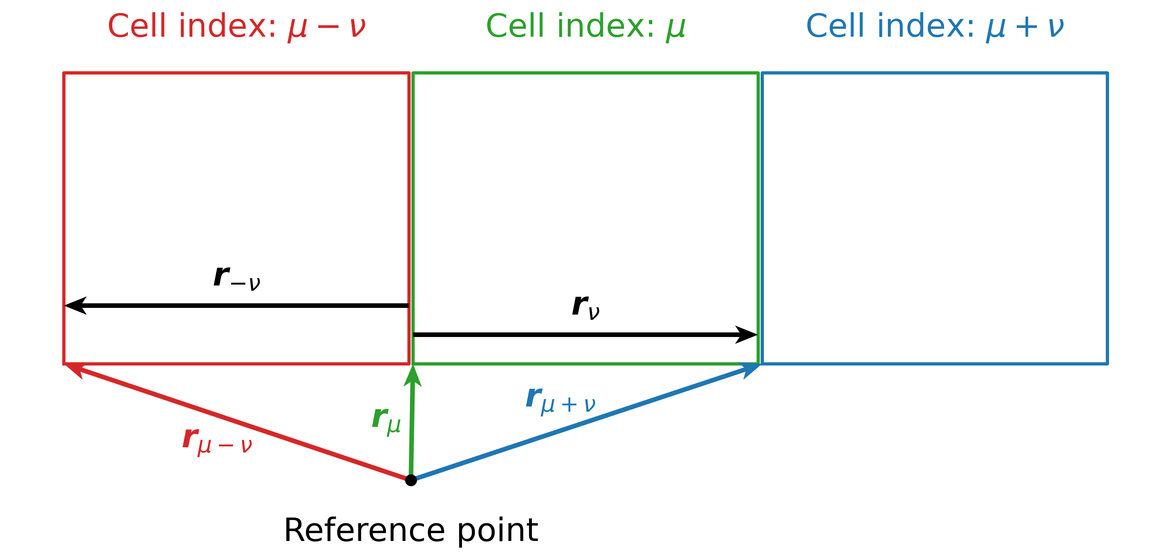
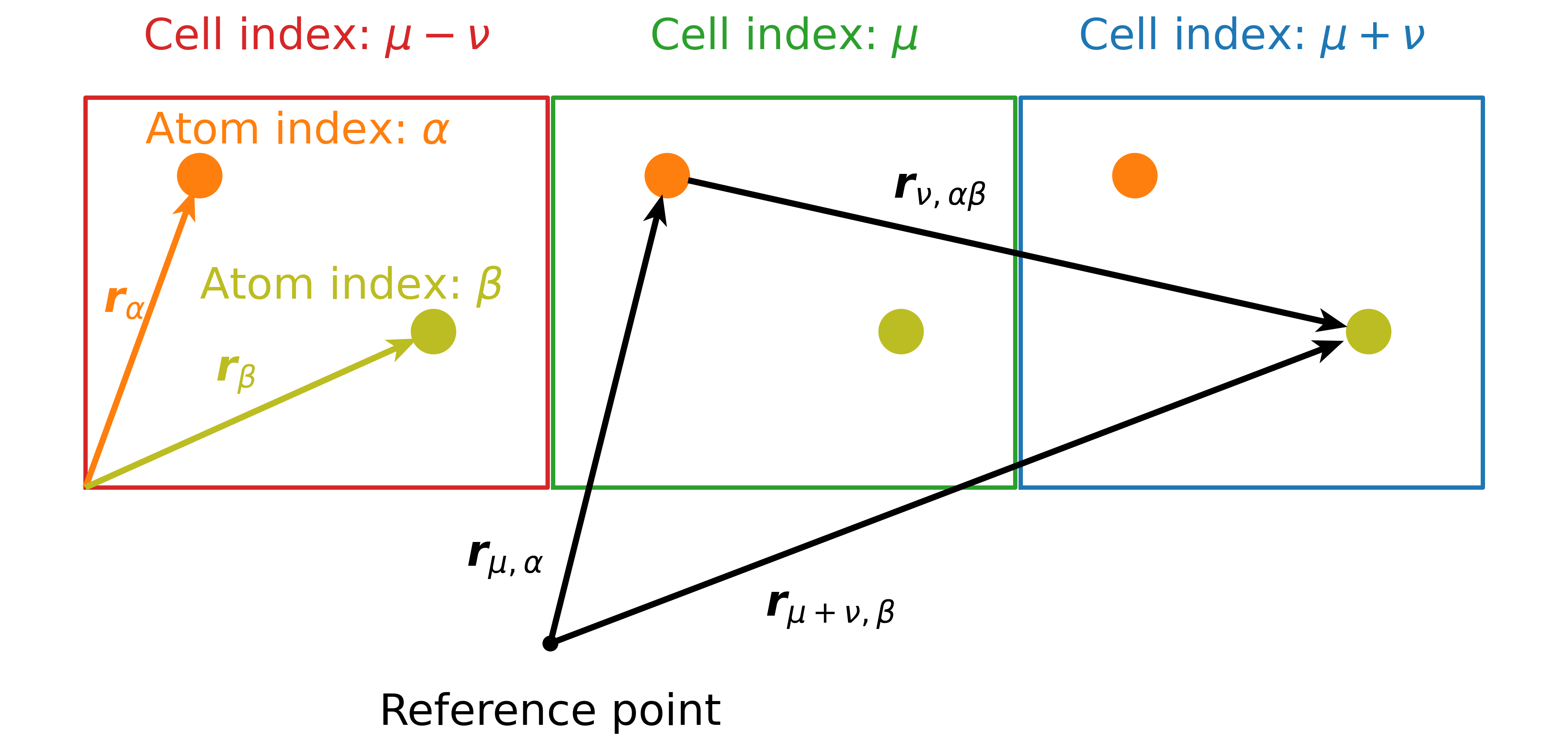
  \[(\boldsymbol{S}_{\mu, \alpha} \cdot \boldsymbol{J}_{\alpha}) = \sum_k S^i_{\mu, \alpha} \cdot J^i_{\alpha}\]

• Subscript Greek letters denote the position of the unit cell in the periodic crystal (\(\mu, \nu, \lambda, \rho\)) or position of the spin within some unit cell (\(\alpha, \beta, \gamma, \varepsilon\)). We understand that the indices \(\mu\) and \(\nu\) (for an 3-dimensional lattice) can be represented by the vector of integer scalars

  \[\begin{split}\mu &= (\mu_1, \mu_2,, \mu_3) \\ \nu &= (\nu_1, \nu_2,, \nu_3)\end{split}\]

  Then the position of the unit cell that contains the spin \(\boldsymbol{S}_{\mu,\alpha}\) is expressed as

  \[\boldsymbol{r}_{\mu} = \sum_{n=1}^3 \mu_n\boldsymbol{a}_n\]

  and the position of the second unit cell that contains the spin \(\boldsymbol{S}_{\mu+\nu,\beta}\) is

  \[\boldsymbol{r}_{\mu + \nu} = \sum_{i=n}^3 (\mu_n + \nu_n)\boldsymbol{a}_n = \boldsymbol{r}_{\mu} + \boldsymbol{r}_{\nu}.\]

  where \(\boldsymbol{a}_n\) are the three lattice vectors of the Bravais lattice of the underlying crystal. In other word the summation and addition of this indices directly translates into the summation and addition of the corresponding position vectors. Note, hat the indices \(\alpha\) and \(\beta\) can be represented by the vectors of three real numbers \(\in [0, 1]\).

  We hope that three images below will help to understand the Greek indices better (click to enlarge)

  

  

The parameters \(\boldsymbol{J}(\boldsymbol{r}_{\alpha})\), \(\boldsymbol{J}(\boldsymbol{r}_{\nu,\alpha\beta})\), \(\boldsymbol{J}(\boldsymbol{r}_{\nu,\alpha\beta}, \boldsymbol{r}_{\lambda,\alpha\gamma})\) and \(\boldsymbol{J}(\boldsymbol{r}_{\nu,\alpha\beta}, \boldsymbol{r}_{\lambda,\alpha\gamma}, \boldsymbol{r}_{\rho,\alpha\varepsilon})\) can describe either some external effect or internal interactions between spins. The Hamiltonian above is discussed and solved in the (TODO) research paper about magnopy.

Expanded form

However, internally and as a part of public API magnopy stores the Hamiltonian in the expanded form

\[\begin{split}\mathcal{H} =& \,C_1 \sum_{\substack{\mu, \\ \alpha \\ i}} J_1^i(\boldsymbol{r}_{\alpha}) S_{\mu,\alpha}^i +\\&+ C_{2,1} \sum_{\substack{\mu, \\ \alpha, \\ i,j}} J_{2,1}^{ij}(\boldsymbol{r}_{\alpha}) S_{\mu,\alpha}^i S_{\mu,\alpha}^j +\\&+ C_{2,2} \sum_{\substack{\mu,\nu, \\ \alpha, \beta, \\ i,j}} J_{2,2}^{ij}(\boldsymbol{r}_{\nu,\alpha\beta}) S_{\mu,\alpha}^i S_{\mu+\nu,\beta}^j +\\&+ C_{3, 1} \sum_{\substack{\mu, \\ \alpha, \\ i,j,u}} J_{3, 1}^{iju}(\boldsymbol{r}_{\alpha}) S_{\mu,\alpha}^i S_{\mu,\alpha}^j S_{\mu,\alpha}^u +\\&+ C_{3, 2} \sum_{\substack{\mu,\nu, \\ \alpha,\beta, \\ i,j,u}} J_{3, 2}^{iju}(\boldsymbol{r}_{\nu,\alpha\beta}) S_{\mu,\alpha}^i S_{\mu,\alpha}^j S_{\mu+\nu,\beta}^u +\\&+ C_{3, 3} \sum_{\substack{\mu,\nu,\lambda, \\ \alpha,\beta,\gamma, \\ i,j,u}} J_{3, 3}^{iju}(\boldsymbol{r}_{\nu,\alpha\beta}, \boldsymbol{r}_{\lambda,\alpha\gamma}) S_{\mu,\alpha}^i S_{\mu+\nu,\beta}^j S_{\mu+\lambda,\gamma}^u +\\&+ C_{4, 1} \sum_{\substack{\mu, \\ \alpha, \\ i,j,u,v}} J_{4, 1}^{ijuv}(\boldsymbol{r}_{\alpha}) S_{\mu,\alpha}^i S_{\mu,\alpha}^j S_{\mu,\alpha}^u S_{\mu,\alpha}^v +\\&+ C_{4, 2, 1} \sum_{\substack{\mu,\nu, \\ \alpha,\beta, \\ i,j,u,v}} J_{4, 2, 1}^{ijuv}(\boldsymbol{r}_{\nu,\alpha\beta}) S_{\mu,\alpha}^i S_{\mu,\alpha}^j S_{\mu,\alpha}^u S_{\mu+\nu,\beta}^v +\\&+ C_{4, 2, 2} \sum_{\substack{\mu,\nu, \\ \alpha,\beta, \\ i,j,u,v}} J_{4, 2, 2}^{ijuv}(\boldsymbol{r}_{\nu,\alpha\beta}) S_{\mu,\alpha}^i S_{\mu,\alpha}^j S_{\mu+\nu,\beta}^u S_{\mu+\nu,\beta}^v +\\&+ C_{4, 3} \sum_{\substack{\mu,\nu,\lambda, \\ \alpha,\beta,\gamma, \\ i,j,u,v}} J_{4, 3}^{ijuv}(\boldsymbol{r}_{\nu,\alpha\beta}, \boldsymbol{r}_{\lambda,\alpha\gamma}) S_{\mu,\alpha}^i S_{\mu,\alpha}^j S_{\mu+\nu,\beta}^u S_{\mu+\lambda,\gamma}^v +\\&+ C_{4, 4} \sum_{\substack{\mu,\nu,\lambda,\rho, \\ \alpha,\beta,\gamma,\varepsilon, \\ i,j,u,v}} J_{4, 4}^{ijuv}(\boldsymbol{r}_{\nu,\alpha\beta}, \boldsymbol{r}_{\lambda,\alpha\gamma}, \boldsymbol{r}_{\rho,\alpha\varepsilon}) S_{\mu,\alpha}^i S_{\mu+\nu,\beta}^j S_{\mu+\lambda,\gamma}^u S_{\mu+\rho,\varepsilon}^v\end{split}\]

Expanded form look monstrous, but it is more convenient as the terms with the same amount of spins, but different number of unique sites can represent distinct physical properties or interactions. Moreover, often the numerical constants before the sum for those terms are different. For example, the on-site quadratic anisotropy is often written with \(C_{2,1} = \pm1\) and bilinear exchange interaction with \(C_{2,2} = \pm1/2\). Both of them describe interaction with two spins, however, it is impossible to write them in the same form with one constant \(C_2\) without modification of the parameters themselves.

Magnopy can read this spin Hamiltonian from TB2J or GROGU automatically, taking into account the convention of the Hamiltonian of each source. Real constants \(C_1\), \(C_{2,1}\), \(C_{2,2}\), \(C_{3,1}\), \(C_{3,2}\), \(C_{3,3}\), \(C_{4,1}\), \(C_{4,2,1}\), \(C_{4,2,2}\), \(C_{4,3}\), \(C_{4,4}\) allow magnopy to support any convention of the spin Hamiltonian. To read more about what defines the convention of the spin Hamiltonian go here.

In the SpinHamiltonian class, that is used to store the parameters of the Hamiltonian, each term is referenced by the numerical indices of the constants. For example, to have access to the third term (two spins & two sites) one can use SpinHamiltonian.p22 property. To add or remove parameters of this term one should use SpinHamiltonian.add_22() and SpinHamiltonian.remove_22().

Examples

In this part we show how the common terms of the spin Hamiltonian can be written in the expanded form.

Zeeman interaction

Linear coupling with the magnetic field is usually written as

\[\mathcal{H} = \mu_B\boldsymbol{h}\sum_{\mu,\alpha} g_a \boldsymbol{S}_{\mu, \alpha}\]

This term can be written as the first term of the expanded form if one defines \(C_1 = 1\) and \(\boldsymbol{J}_1(\boldsymbol{r}_{\alpha}) = \mu_B\boldsymbol{h} g_a\).

On-site anisotropy

We take an example of the triaxial anisotropy, that can be written as

\[\mathcal{H} = \sum_{\mu,\alpha} \Bigl( K^x (S^x_{\mu,\alpha})^2 + K^y (S^y_{\mu,\alpha})^2 + K^z (S^z_{\mu,\alpha})^2 \Bigr)\]

This Hamiltonian can be written as the second term of the expanded form if one defines \(C_{2,1} = 1\) and

\[\begin{split}\boldsymbol{J}_{2,1}(\boldsymbol{r}_{\alpha}) = \begin{pmatrix} K^x & 0 & 0 \\ 0 & K^y & 0 \\ 0 & 0 & K^z \end{pmatrix}\end{split}\]

Exchange interaction

Bilinear exchange interaction with isotropic and Dzyaloshinskii-Moriya (DM) exchange can be written as

\[\mathcal{H} = \dfrac{1}{2} \sum_{\mu,\alpha} \sum_{\mu + \nu,\beta} \Bigl[ J^{iso}(\boldsymbol{r}_{\nu,\alpha\beta}) (\boldsymbol{S}_{\mu,\alpha} \cdot \boldsymbol{S}_{\mu+\nu,\beta}) + \boldsymbol{D}(\boldsymbol{r}_{\nu,\alpha\beta}) \cdot (\boldsymbol{S}_{\mu,\alpha} \times \boldsymbol{S}_{\mu+\nu,\beta}) \Bigr]\]

where \(\boldsymbol{D}(\boldsymbol{r}_{\nu,\alpha\beta})\) is a DM vector. This Hamiltonian can be written as the third term of the expanded form if one defines \(C_{2,2} = 1/2\) and

\[\begin{split}J_{2,2}(\boldsymbol{r}_{\nu,\alpha\beta}) = \begin{pmatrix} J^{iso}(\boldsymbol{r}_{\nu,\alpha\beta}) & D^z(\boldsymbol{r}_{\nu,\alpha\beta}) & -D^y(\boldsymbol{r}_{\nu,\alpha\beta}) \\ -D^z(\boldsymbol{r}_{\nu,\alpha\beta}) & J^{iso}(\boldsymbol{r}_{\nu,\alpha\beta}) & D^x(\boldsymbol{r}_{\nu,\alpha\beta}) \\ D^y(\boldsymbol{r}_{\nu,\alpha\beta}) & -D^x(\boldsymbol{r}_{\nu,\alpha\beta}) & J^{iso}(\boldsymbol{r}_{\nu,\alpha\beta}) \end{pmatrix}\end{split}\]

Biquadratic exchange

Isotropic biquadratic exchange interaction can be written as

\[\mathcal{H} = \sum_{\mu,\alpha} \sum_{\mu + \nu,\beta} J(\boldsymbol{r}_{\nu,\alpha\beta}) (\boldsymbol{S}_{\mu,\alpha} \cdot \boldsymbol{S}_{\mu+\nu,\beta})^2\]

This Hamiltonian can be written as the ninth term of the expanded form is one defines \(C_{4,2,2} = 1\) and tensor \(\boldsymbol{J}_{4,2,2}(\boldsymbol{r}_{\nu,\alpha\beta})\) such as \(J_{4,2,2}^{ijuv}(\boldsymbol{r}_{\nu,\alpha\beta}) = J(\boldsymbol{r}_{\nu,\alpha\beta})\) if \((ijuv)\) is one of

\[\begin{split}\begin{matrix} (xxxx), & (xyxy), & (xzxz), \\ (yxyx), & (yyyy), & (yzyz), \\ (zxzx), & (zyzy), & (yyyy) \end{matrix}\end{split}\]

and \(J_{4,2,2}^{ijuv}(\boldsymbol{r}_{\nu,\alpha\beta}) = 0\) otherwise.